The rise of Large Language Models (LLMs) and other Machine Learning tools such as CLIP and semantic search has made Vector Databases a critical component of modern infrastructure. They are the foundational retrieval engine behind Retrieval-Augmented Generation (RAG), enabling AI applications to dynamically pull relevant, domain-specific context from massive datasets. But unlike traditional databases that search for exact substring matches, vector databases search for meaning.
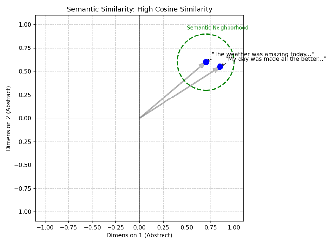
For example, if we vectorize two separate images of a dog in some representation space, we should expect that those vectors should be closer together than the vectors of an image of a dog to that of an image of a car. Similarly, these two sentences embedded into a vector space should be expected to be closer together because they have similar meaning:
The weather was amazing today and made me so happy!
My day was made all the better by the beautiful weather!
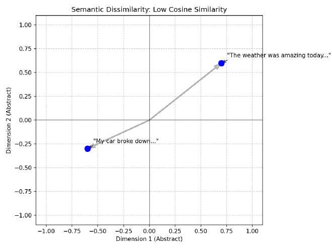
And we should also expect these two sentences to have vector representations that are much further away from each other because their meanings are quite different:
The weather was amazing today and made me so happy!
My car broke down and I got a flat tire on the way to work!
Intuitively this makes sense, but intuition isn’t good enough for computation. So how do we quantify these differences in a scalable, efficient manner?
To do this, we rely on Approximate Nearest Neighbor (ANN) algorithms to navigate high-dimensional spaces efficiently. This post provides an introduction to the core algorithms that empower embedding vector searching at scale.
TL;DR: The 60-Second Summary#
- The Problem: High-dimensional math breaks traditional spatial trees (like KD-Trees). Distances “concentrate”, making everything look equidistant, meaning you have to scan the whole database anyway.
- The Engine: HNSW (Hierarchical Navigable Small World) is the common default for in-memory search, using a multi-layered proximity graph (think Skip Lists but in a graph) to route queries in expected $O(\log N)$ time.
- The Scaling Challenge: HNSW uses massive amounts of RAM (often costing hundreds of bytes to a couple KB/vector depending on ID width, $M$, and implementation). At billion-scale, this is often cost-prohibitive to keep entirely in memory.
- The Solutions:
- Quantization (PQ/SQ): Compress the vectors severely (e.g., PQ: 384 float32 → 48 bytes) to fit them in RAM, at the cost of slight recall loss.
- DiskANN: A graph designed explicitly for fast NVMe SSD reads, typically reducing RAM needs by ~10x-100x vs naive in-memory graphs, depending on PQ and caching.
- Sparse Vectors: Lexical vectors (like BM25 or SPLADE) are 99% zeros and run on entirely different infrastructure (Inverted Indexes) rather than the ANN pipelines described here. Sparse vectors have different failure modes; inverted indexes avoid the same geometry-driven pruning collapse.
Note: Code blocks in this document are minimal for conceptual clarity; some explicitly omit imports, memory management, and structural boilerplate.
Out of Scope: Dense vs. Sparse Vectors#
This post exclusively covers the mathematics of Dense Vector Search.
Dense vectors (like embeddings from OpenAI or CLIP) have hundreds to a few thousand dimensions (far lower than sparse vocab-scale vectors). Dense embeddings require evaluating similarity across (nearly) all dimensions, so high-dimensional geometry and distance concentration matter operationally.
By contrast, Sparse Vectors (such as traditional TF-IDF/BM25 profiles, or modern neural representations like SPLADE [splade-paper] and Elastic’s ELSER) have massive dimensionality (often corresponding to the entire English vocabulary, e.g., 30,000+ dimensions), but they are 99% zeros. Sparse retrieval typically exploits Inverted Indexes (data structures that map terms directly to the list of documents containing them) so scoring touches only non-zero coordinates, changing both the cost model and failure modes. Therefore, sparse vectors do not suffer from the same geometric curse, and algorithms like HNSW or IVF are not the primary mechanisms for scaling them.
The Classical Approach: Space Partitioning#
Before we had modern vector databases or graph algorithms, we had spatial indexes. In low-dimensional spaces (like 2D maps or 3D CAD models), we solved the nearest neighbor problem using Space Partitioning Trees:
KD-Trees (k-dimensional Trees)#
A KD-Tree is a binary tree that splits the data space into two halves at every node using axis-aligned hyperplanes (hyperplanes are just n-dimensional planes).
- Root: Split the data along the X-axis (dimension 0) at the median. Points with $x < median$ go left; points with $x \ge median$ go right.
- Level 1: Split each child node along the Y-axis (dimension 1). Notice in the diagram below that the split values (e.g., $Y < 30$ vs $Y < 80$) are different for each branch because they are the local medians for that specific subset of points.
- Level 2: Split along the Z-axis (dimension 2), and so on, cycling through dimensions.
class Node:
    def __init__(self, point, left=None, right=None, axis=0):
        self.point = point
        self.left = left
        self.right = right
        self.axis = axis

def build_kdtree(points, depth=0):
    if not points:
        return None

    k = len(points[0])  # dimensionality
    axis = depth % k    # cycle through axes

    # Sort points and choose median (we copy to avoid mutating the input array)
    points = points.copy()
    points.sort(key=lambda x: x[axis])
    median = len(points) // 2

    # Note: For production, prefer `nth_element`/partition selection and
    # operate on index ranges to avoid repeated sorts (which push toward O(N log^2 N)) and avoid copying slices (which causes heavy memory churn).
    return Node(
        point=points[median],
        left=build_kdtree(points[:median], depth + 1),
        right=build_kdtree(points[median + 1:], depth + 1),
        axis=axis
    )
type Node struct {
    Point []float64
    Left  *Node
    Right *Node
    Axis  int
}

func BuildKDTree(points [][]float64, depth int) *Node {
    if len(points) == 0 {
        return nil
    }

    k := len(points[0])
    axis := depth % k

    // Sort by current axis (simplified)
    sort.Slice(points, func(i, j int) bool {
        return points[i][axis] < points[j][axis]
    })

    median := len(points) / 2
    return &Node{
        Point: points[median],
        Left:  BuildKDTree(points[:median], depth+1),
        Right: BuildKDTree(points[median+1:], depth+1),
        Axis:  axis,
    }
}
struct Node {
    std::vector<double> point;
    Node *left = nullptr;
    Node *right = nullptr;
    int axis;

    Node(std::vector<double> pt, int ax) : point(pt), axis(ax) {}
};

Node* buildKDTree(std::vector<std::vector<double>>& points, int depth) {
    if (points.empty()) return nullptr;

    int axis = depth % points[0].size();
    int median = points.size() / 2;

    // Use nth_element to find median in O(N)
    std::nth_element(points.begin(), points.begin() + median, points.end(),
        [axis](const auto& a, const auto& b) { return a[axis] < b[axis]; });

    Node* node = new Node(points[median], axis);

    std::vector<std::vector<double>> leftPoints(points.begin(), points.begin() + median);
    std::vector<std::vector<double>> rightPoints(points.begin() + median + 1, points.end());

    node->left = buildKDTree(leftPoints, depth + 1);
    node->right = buildKDTree(rightPoints, depth + 1);

    return node;
}
Search: To find the nearest neighbor, you traverse the tree from root to leaf (expected $\log N$ steps). You can prune entire branches of the tree if the query point is too far from the bounding box of that branch. In low dimensions ($d < 10$), this is incredibly efficient (expected / empirical under typical assumptions; worst-case can degrade).
KD-Trees vs. Prefix Trees: While KD-Trees partition continuous geometric space by splitting along dimensional medians, you might also hear about Prefix Trees (Tries or Radix Trees). Prefix Trees partition discrete data (like strings or bitwise representations) by their structural prefixes. They are fundamentally built for exact or longest-prefix matching rather than spatial nearest-neighbor approximations. For a deep dive into $O(L)$ digital search complexity, see our dedicated post on The Architecture of Prefix Trees.
R-Trees (Rectangle Trees): Object-Centric Grouping#
While KD-Trees partition the space (splitting the canvas like a grid, regardless of where the data is), R-Trees (where “R” stands for “Rectangle”) partition the data (grouping the ink, drawing boxes only where the points actually exist).
The Core Concept: Minimum Bounding Rectangles (MBRs) An R-Tree groups nearby objects into a box described by its coordinates: $(min_x, min_y)$ and $(max_x, max_y)$.
- Leaf Nodes: Contain actual data points.
- Internal Nodes: Contain the “MBR” that encompasses all its children.
The Fatal Flaw: Overlap Unlike KD-Trees, where a single median hyperplane strictly divides the space into infinitely disjoint halves, R-Trees draw boxes dynamically around point clusters. Because these clusters grow organically and aren’t bounded by a global grid, the Minimum Bounding Rectangles of sibling nodes can (and frequently do) physically overlap in space. If a query point falls into an overlapping region, it intersects the bounding boxes of multiple sibling nodes, forcing the algorithm to search down multiple paths.
- Low Dimensions: Overlap is minimal; search remains expected $O(\log N)$ under typical assumptions (worst-case can degrade).
- High Dimensions: As dimensions rise, the “empty space” problem forces MBRs to grow larger to encompass their children. Eventually, MBRs overlap significantly. A single query might intersect with 50% of the tree’s branches, destroying the pruning advantage.
Search Logic: You calculate which MBRs intersect with your query’s search radius. You must descend into every intersecting MBR.
class MBR:
    def __init__(self, min_coords, max_coords):
        self.min = min_coords  # [x_min, y_min, ...]
        self.max = max_coords  # [x_max, y_max, ...]

    def intersects(self, query_point, radius):
        # Accumulate squared distances across ALL dimensions
        dist_sq = 0
        for i in range(len(query_point)):
            # Per-dimension distance to the box
            delta = 0
            if query_point[i] < self.min[i]:
                delta = self.min[i] - query_point[i]
            elif query_point[i] > self.max[i]:
                delta = query_point[i] - self.max[i]
            dist_sq += delta * delta
        return dist_sq <= radius * radius
type MBR struct {
    Min []float64
    Max []float64
}

func (m MBR) Intersects(query []float64, radius float64) bool {
    distSq := 0.0
    for i := range query {
        delta := 0.0
        if query[i] < m.Min[i] {
            delta = m.Min[i] - query[i]
        } else if query[i] > m.Max[i] {
            delta = query[i] - m.Max[i]
        }
        distSq += delta * delta
    }
    return distSq <= radius*radius
}
struct MBR {
    std::vector<double> min_coords;
    std::vector<double> max_coords;

    bool intersects(const std::vector<double>& query, double radius) {
        double dist_sq = 0.0;
        for (size_t i = 0; i < query.size(); ++i) {
            double delta = 0.0;
            if (query[i] < min_coords[i]) {
                delta = min_coords[i] - query[i];
            } else if (query[i] > max_coords[i]) {
                delta = query[i] - max_coords[i];
            }
            dist_sq += delta * delta;
        }
        return dist_sq <= radius * radius;
    }
};
The Failure Mode: Why Pruning Fails in High Dimensions#
What is Pruning? In a search tree, “pruning” means safely ignoring an entire branch of the tree. If you know for a fact that the closest point in a branch is 10 units away, but you’ve already found a neighbor that is 5 units away, you don’t need to enter that branch at all. You “prune” it.
Deriving $O(\log N)$ Search Complexity: Let $N$ be the total number of data points and $B$ be the structural branching factor of the tree (e.g., $B=2$ for a binary KD-Tree). Assuming uniform distribution, the root node contains $N$ points, its children contain $N/B$ points, and at depth $h$, a node contains $N/B^h$ points. The tree reaches its deepest leaf when a node contains exactly $1$ point ($N/B^h = 1$). Solving for $h$ yields $B^h = N$, deriving the maximum height of a balanced tree as $h = \log_B(N)$.
During a nearest-neighbor search, if geometric properties allow the algorithm to confidently prune all but a small constant number of branches $C$ at each descended level, the total number of nodes evaluated is at most $C \cdot h$. Therefore, the overall search complexity is formally bounded by $O(C \cdot \log_B N)$, which simplifies asymptotically to $O(\log N)$.
(Note: The “Curse of Dimensionality” occurs when pruning fails and $C$ approaches $B$. Even if $B$ is a small constant (like $B=2$ in a KD-Tree), being forced to evaluate $B$ branches out of $B$ total possibilities at every level means you are traversing the entire graph ($O(B^h)$). Since $B^h = N$, the search fatally degrades to $O(N)$).
Classical High-Dimensional Attempts: LSH & Random Projections#
As practitioners realized trees failed in high dimensions, the classical “theory-first” approach shifted to Locality Sensitive Hashing (LSH). Rooted in the Johnson-Lindenstrauss lemma (which provides the intuition that random projections approximately preserve pairwise distances [jl-lemma-proof]), LSH uses random hyperplanes to hash vectors into buckets.
If two vectors are close in space, they are highly likely to fall on the same side of a random hyperplane, and thus land in the same hash bucket. Random hyperplane LSH specifically targets cosine (angular) distance [charikar-simhash]. While mathematically elegant, LSH requires many parallel hash tables to achieve good recall and struggles with precision compared to the modern graph-based methods we use today.
Another historical parallel is Random Projection Forests (e.g., Annoy). Popularized by Spotify, algorithms like Annoy build a “forest” of trees by recursively splitting the space using random hyperplanes rather than strict axis-aligned ones. You search multiple trees simultaneously to find the nearest neighbor. Annoy is historically famous and excellent for simple memory-mapped workloads, but its performance curve is largely dwarfed by HNSW and ScaNN today.
The “High-Dimensional” Problem In 2D or 3D, space is “crowded” and data points are distinct. If you are in one quadrant, you are far from the others. However, as dimensions increase ($D > 10$), a strange geometric phenomenon occurs: points move to the edges [aggarwal-surprising].
Imagine a high-dimensional hypercube. The volume of the cube is $1^D$. The volume of a slightly smaller inscribed cube (say, 90% size) is $0.9^D$.
- In 2D: $0.9^2 = 0.81$ (81% of volume is in the center).
- In 100D: $0.9^{100} \approx 0.00002$ (Almost 0% of volume is in the center!).
The Consequence: Almost all data points sit on the “surface” or shell of the structure. When you query this space:
- Your query point is almost always near a “boundary” of the partition.
- The “search radius” effectively overlaps with every partition.
- You cannot prove that a branch is “too far away” because in high dimensions, relative distance contrast collapses (nearest and farthest distances concentrate), so ‘close vs far’ becomes hard to separate.
Because you can’t rule out any branches, you are forced to visit them all. The tree devolves into a complicated, slow linked list, often performing worse than a brute-force linear scan.
The Challenge: The Curse of Dimensionality#
Before diving into the solutions, we must understand the problem. Why can’t we just use a B-Tree or a KD-Tree?
B-trees index ordered keys; nearest-neighbor in vector spaces isn’t naturally representable as a total order. For low-dimensional spaces (like 2D or 3D geographical data), structures like KD-Trees or R-Trees work beautifully. They partition space so you can quickly discard vast regions that are “too far away.”
However, modern embedding models (like CLIP or OpenAI’s text-embedding-3) output vectors with hundreds or thousands of dimensions (e.g., 512, 768, 1536, or 3072). In these high-dimensional spaces, a phenomenon known as the Curse of Dimensionality renders traditional spatial partitioning ineffective.
Mathematically, as dimension $D$ increases:
- Distance Concentration [aggarwal-surprising]: The ratio of the distance to the nearest neighbor vs. the farthest neighbor approaches 1. Relative distance contrast collapses (nearest and farthest distances concentrate), so ‘close vs far’ becomes hard to separate, making it impossible for the algorithm to distinguish a “clear” winner.
- Empty Space: As discussed in the Failure Mode section above, volume expands exponentially, pushing all data points to the surface.
The “Dice Roll” Intuition: Think of 1 dimension as rolling a single die. You can easily get a 1 (min) or a 6 (max). The “contrast” is high. Now, think of 1,000 dimensions as summing 1,000 independent dice. According to the Central Limit Theorem, the sum of independent random variables tends toward a Normal Distribution (Gaussian). The result will cluster tightly around the mean (3,500). It is effectively statistically impossible to roll all 1s (1,000) or all 6s (6,000). In high dimensions, every vector is effectively a “sum of many dice.” Its length (norm) and distance to others converge to a statistical mean. The “spikes” (unique features) get washed out in the law of large numbers.
The Saving Grace: Intrinsic Dimension While the math above assumes embeddings are perfectly uniform across all dimensions, real-world data is inherently structured. Embeddings typically lie on much lower-dimensional manifolds (their intrinsic dimension is much smaller than their raw dimension $D$). This clustered, non-uniform structure is the saving grace that allows ANN algorithms to successfully partition and navigate the space despite the raw geometric curse.
The Hubness Phenomenon Because of that same high-dimensional concentration, embedding spaces also exhibit “Hubness.” A very small subset of dense vectors (the “hubs”) end up appearing as the nearest neighbors for a large fraction of uncorrelated queries [hubness-radovanovic], which requires careful algorithm tuning to avoid retrieving the same dominant hubs over and over.
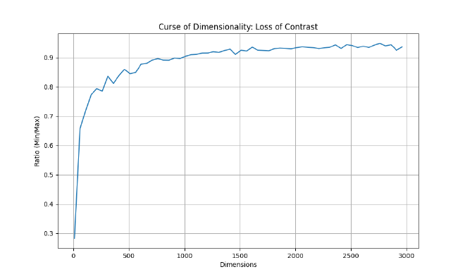
To visualize this, here is a script to generate the “Ratio of Distances” graph shown above.
import numpy as np
import matplotlib.pyplot as plt

# Seed RNG for deterministic notebook reproducibility
np.random.seed(42)

def calculate_ratio(dim, num_points=1000):
    # Generate random points on unit sphere
    points = np.random.randn(num_points, dim)
    points /= np.linalg.norm(points, axis=1)[:, np.newaxis]

    # Calculate min/max pairwise distances
    # (Approximation: compare 1st point to all others to save time;
    # the true min/max would check all pairs, but this serves the intuition)
    diff = points[1:] - points[0]
    dists = np.linalg.norm(diff, axis=1)

    return np.min(dists) / np.max(dists)

dims = range(10, 3001, 50)
ratios = [calculate_ratio(d) for d in dims]

plt.figure(figsize=(10, 6))
plt.plot(dims, ratios, label='Min/Max Distance Ratio')
plt.xlabel('Dimensions')
plt.ylabel('Ratio (Min/Max)')
plt.title('Curse of Dimensionality: Loss of Contrast')
plt.grid(True)
plt.savefig('curse_of_dimensionality.png')
print("Graph saved to curse_of_dimensionality.png")
package main

import (
	"fmt"
	"math"
	"math/rand"
)

func calculateRatio(rng *rand.Rand, dim, numPoints int) float64 {
	points := make([][]float64, numPoints)
	for i := range points {
		points[i] = make([]float64, dim)
		var norm float64
		for j := 0; j < dim; j++ {
			v := rng.NormFloat64()
			points[i][j] = v
			norm += v * v
		}
		norm = math.Sqrt(norm)
		for j := 0; j < dim; j++ {
			points[i][j] /= norm
		}
	}

	minDist, maxDist := math.MaxFloat64, 0.0

	// Compare point 0 to all others
	for i := 1; i < numPoints; i++ {
		var distSq float64
		for k := 0; k < dim; k++ {
			diff := points[0][k] - points[i][k]
			distSq += diff * diff
		}
		dist := math.Sqrt(distSq)
		if dist < minDist {
			minDist = dist
		}
		if dist > maxDist {
			maxDist = dist
		}
	}

	return minDist / maxDist
}

func main() {
	rng := rand.New(rand.NewSource(42))
	for dim := 10; dim <= 3000; dim += 50 {
		ratio := calculateRatio(rng, dim, 1000)
		fmt.Printf("%d,%.4f\n", dim, ratio)
	}
}
#include <iostream>
#include <vector>
#include <random>
#include <cmath>
#include <algorithm>
#include <iomanip>

double calculate_ratio(int dim, int num_points = 1000) {
    std::vector<std::vector<double>> points(num_points, std::vector<double>(dim));
    std::mt19937 gen(42);
    std::normal_distribution<> d(0, 1);

    for (int i = 0; i < num_points; ++i) {
        double norm_sq = 0.0;
        for (int j = 0; j < dim; ++j) {
            points[i][j] = d(gen);
            norm_sq += points[i][j] * points[i][j];
        }
        double norm = std::sqrt(norm_sq);
        for (int j = 0; j < dim; ++j) {
            points[i][j] /= norm;
        }
    }

    double min_dist = 1e9;
    double max_dist = 0.0;

    // Compare point 0 to all others
    for (int i = 1; i < num_points; ++i) {
        double dist_sq = 0.0;
        for (int k = 0; k < dim; ++k) {
            double diff = points[0][k] - points[i][k];
            dist_sq += diff * diff;
        }
        double dist = std::sqrt(dist_sq);
        min_dist = std::min(min_dist, dist);
        max_dist = std::max(max_dist, dist);
    }
    return min_dist / max_dist;
}

int main() {
    std::cout << "dimension,ratio\n";
    for (int dim = 10; dim <= 3000; dim += 50) {
        double ratio = calculate_ratio(dim);
        std::cout << dim << "," << std::fixed << std::setprecision(4) << ratio << "\n";
    }
    // Pipe this output to a plotting tool
    return 0;
}
This forces us to compromise: we trade exactness for speed, accepting “approximate” nearest neighbors (ANN) to achieve sub-linear search times.
Distance Metrics: The Foundation#
Baseline: Linear Search (Exact k-NN)#
Before optimizing, it’s useful to know the baseline. This is the $O(N)$ approach.
Production Context: While too slow for billion-scale data, this brute-force approach guarantees 100% recall. Providers often expose this explicitly (e.g., Azure AI Search calls its brute-force algorithm
exhaustiveKnn[azure-ai-search-vector-index]) for use cases requiring absolute precision on small, pre-filtered datasets, or to generate a gold-standard ground truth for evaluating ANN recall.
import numpy as np

def linear_search(query, dataset):
    best_dist = float('inf')
    best_item = None

    for item in dataset:
        dist = np.linalg.norm(query - item)
        if dist < best_dist:
            best_dist = dist
            best_item = item

    return best_item, best_dist
func LinearSearch(query []float64, dataset [][]float64) ([]float64, float64) {
	bestDist := math.MaxFloat64
	var bestItem []float64

	for _, item := range dataset {
		dist := EuclideanDistance(query, item)
		if dist < bestDist {
			bestDist = dist
			bestItem = item
		}
	}
	return bestItem, bestDist
}
#include <vector>
#include <limits>
#include <cmath>

std::pair<std::vector<double>, double> linear_search(const std::vector<double>& query, const std::vector<std::vector<double>>& dataset) {
    double best_dist = std::numeric_limits<double>::max();
    std::vector<double> best_item;

    for (const auto& item : dataset) {
        double dist = euclidean_distance(query, item);
        if (dist < best_dist) {
            best_dist = dist;
            best_item = item;
        }
    }
    return {best_item, best_dist};
}
All ANN algorithms operate on a distance (or similarity) function between vectors. The choice of metric affects both the mathematics of the index and the quality of retrieval results.
Euclidean Distance (L2)#
Measures the straight-line distance between two points in $\mathbb{R}^d$:
$$d_{\text{L2}}(\mathbf{x}, \mathbf{y}) = \sqrt{\sum_{i=1}^{d} (x_i - y_i)^2}$$
Cosine Similarity#
Measures the angle between two vectors, normalized to [-1, 1]. It effectively ignores the magnitude of the vectors, focusing only on their direction (semantic meaning).
$$\text{cos}(\mathbf{x}, \mathbf{y}) = \frac{\mathbf{x} \cdot \mathbf{y}}{|\mathbf{x}| \cdot |\mathbf{y}|} = \frac{\sum_{i=1}^{d} x_i y_i}{\sqrt{\sum_{i=1}^{d} x_i^2} \cdot \sqrt{\sum_{i=1}^{d} y_i^2}}$$
Inner Product (IP / Dot Product)#
Inner product (dot product) is used for Maximum Inner Product Search (MIPS). If vectors are unit-normalized, dot product ranking exactly matches cosine similarity:
$$\text{IP}(\mathbf{x}, \mathbf{y}) = \sum_{i=1}^{d} x_i y_i$$
import numpy as np

def cosine_similarity(v1, v2):
    dot_product = np.dot(v1, v2)
    norm_v1 = np.linalg.norm(v1)
    norm_v2 = np.linalg.norm(v2)
    return dot_product / (norm_v1 * norm_v2)
func CosineSimilarity(v1, v2 []float64) float64 {
	var dot, norm1, norm2 float64
	for i := range v1 {
		dot += v1[i] * v2[i]
		norm1 += v1[i] * v1[i]
		norm2 += v2[i] * v2[i]
	}
	if norm1 == 0 || norm2 == 0 {
		return 0
	}
	return dot / (math.Sqrt(norm1) * math.Sqrt(norm2))
}
#include <vector>
#include <cmath>

double cosine_similarity(const std::vector<double>& v1, const std::vector<double>& v2) {
    double dot = 0.0, norm1 = 0.0, norm2 = 0.0;
    for (size_t i = 0; i < v1.size(); ++i) {
        dot += v1[i] * v2[i];
        norm1 += v1[i] * v1[i];
        norm2 += v2[i] * v2[i];
    }
    if (norm1 == 0 || norm2 == 0) return 0.0;
    return dot / (std::sqrt(norm1) * std::sqrt(norm2));
}
MIPS vs Distance Cheat Sheet: When working with Maximum Inner Product Search (MIPS) and distances, practitioners rely on these canonical reductions:
- L2 to Dot Product Equivalency: If you unit-normalize your vectors ($||x|| = 1$), calculating the Dot Product yields the exact same ranking as computing Cosine Similarity or Euclidean (L2) distance.
- MIPS to L2 Reduction: For unnormalized vectors, MIPS can be converted into an L2 search problem by augmenting the data vectors with an extra dimension $x^\prime = [x; \sqrt{R^2 - ||x||^2}]$ (where $R \ge \max_x ||x||$). The query gets padded with a zero: $q^\prime = [q; 0]$. This ensures $||x^\prime||$ is constant, making finding the minimum L2 distance mathematically equivalent to finding the maximum inner product: $||q^\prime - x^\prime||^2 = ||q||^2 + R^2 - 2(q \cdot x)$.
- Norm Drift: If you rely on dot product as a proxy for cosine, you must enforce normalization; otherwise ranking differences emerge as norms vary, sometimes materially.
Graph-Based Indexing: HNSW#
HNSW (Hierarchical Navigable Small World) [malkov-hnsw] is currently a de facto default for in-memory vector search. It works by constructing a multi-layered proximity graph.
The Small World Phenomenon#
A navigable small world graph has a special property: even though each node connects to only a few neighbors (low degree), the graph is structured so that you can hop between any two nodes in very few steps (empirically near $O(\log N)$ for typical data distributions).
- Intuition: Think of the “Six Degrees of Kevin Bacon.” You can connect any actor to Kevin Bacon in less than 6 steps knowing only who worked with whom.
Multi-Layered Architecture#
HNSW borrows ideas from Skip Lists (a linked list with “express lanes” that let you skip over 10, 50, or 100 items at a time). It builds a hierarchy of graph layers:
- Top Layer (Highways): Very few nodes. Long-range links. Allows you to “zoom” across the vector space quickly (like taking an Interstate highway).
- Middle Layers: More nodes. Finer granularity (like exiting to state routes).
- Bottom Layer (Layer 0): Contains every vector. Used for the final, precise search (like navigating neighborhood streets).
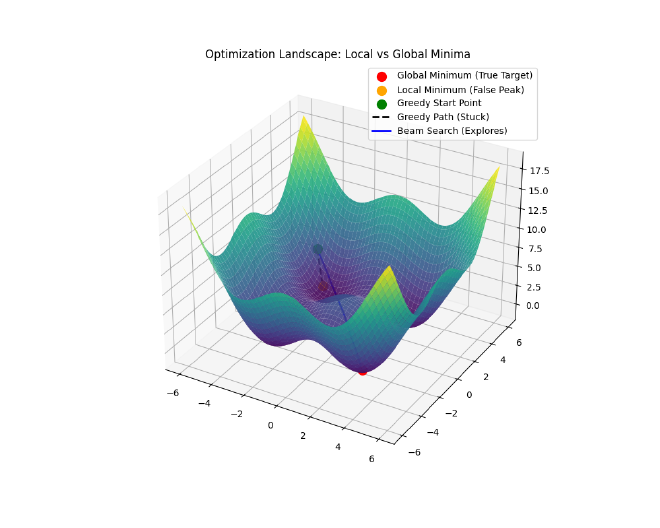
Search Algorithm (Greedy Routing & Beam Search)#
The search uses Greedy Routing with a Beam Search buffer.
- Intuition (Greedy): Imagine driving toward a mountain peak (the Query) you can see in the distance. At every intersection (Node), you turn down the road that points most directly at the peak.
- Intuition (Beam Search): Instead of sending just one car, you send a fleet of $ef$ (Exploration Factor) cars. They explore slightly different routes. If one car hits a dead end (a “local minimum” where all neighbors are further away), the others can still find the peak.
The Algorithm Steps:#
- Enter at the top layer.
- Greedily traverse to the node closest to the query.
- Descend to the next layer, using the current node as the entry point.
- Repeat until Layer 0.
- Beam Search at Layer 0:
- Maintain a priority queue
Wof sizeef(Exploration Factor). Wstores the “best candidates found so far.”- At each step, explore the neighbors of the closest candidate in
W. - Add them to
Wif they are closer than the worst candidate inW(and drop the worst one to keepWat sizeef). - Stop when no candidate in
Wyields a closer neighbor.
- Maintain a priority queue
Mathematical Complexity: Why ~$O(\log N)$?#
Why is HNSW so fast? It comes down to the probability of layer promotion, similar to a Skip List.
HNSW Layer Assignment Logic (Code)#
The core idea is Probabilistic Layer Promotion. Instead of balancing a tree recursively, HNSW relies on an exponential/geometric distribution parameterized by $M$ (the maximum number of neighbors per layer). By taking the negative natural logarithm of a uniform random float and scaling it by $m_L = 1 / \ln(M)$, the probability of a node reaching layer $L$ perfectly decays by a factor of $1/M$ at each step.
import random
import math

class HNSWNode:
    def __init__(self, value, level):
        self.value = value
        # Neighbors list for each layer from 0 to level
        self.neighbors = [[] for _ in range(level + 1)]

class HNSWGraph:
    def __init__(self, M=16, max_level=16):
        self.M = M
        self.max_level = max_level
        # The normalization factor
        self.m_L = 1.0 / math.log(M)

    def random_level(self):
        # HNSW layer assignment follows an exponential distribution.
        # This ensures the probability of reaching layer L decays by 1/M at each step.
        f = random.uniform(0, 1)
        # Avoid log(0) edge case
        if f == 0.0:
            f = 1e-10

        level = int(-math.log(f) * self.m_L)
        return min(level, self.max_level)
package main

import (
	"math"
	"math/rand"
)

type HNSWNode struct {
	Value     int
	Neighbors [][]int // Indexes of neighbors at each layer
}

type HNSWGraph struct {
	M        int
	MaxLevel int
	mL       float64
	rng      *rand.Rand
}

func NewHNSWGraph(m int, maxLevel int, seed int64) *HNSWGraph {
	return &HNSWGraph{
		M:        m,
		MaxLevel: maxLevel,
		mL:       1.0 / math.Log(float64(m)),
		rng:      rand.New(rand.NewSource(seed)),
	}
}

func (g *HNSWGraph) RandomLevel() int {
	// Exponential distribution scaled by 1/ln(M)
	f := g.rng.Float64()
	if f == 0.0 {
		f = 1e-10
	}

	level := int(-math.Log(f) * g.mL)

	if level > g.MaxLevel {
		return g.MaxLevel
	}
	return level
}
#include <vector>
#include <cmath>
#include <random>
#include <algorithm>

struct HNSWNode {
    int value;
    std::vector<std::vector<int>> neighbors; // Neighbors for each layer

    HNSWNode(int v, int level) : value(v), neighbors(level + 1) {}
};

class HNSWGraph {
    int M;
    int max_level;
    double m_L;
    std::mt19937 gen;
    std::uniform_real_distribution<double> dist;

public:
    HNSWGraph(int m, int max_lvl)
        : M(m), max_level(max_lvl), m_L(1.0 / std::log(m)), gen(42), dist(0.0, 1.0) {}

    int randomLevel() {
        // Sample from uniform(0,1), take -ln(), scale by m_L
        double f = dist(gen);
        // Avoid log(0)
        if (f == 0.0) f = 1e-10;

        int lvl = static_cast<int>(-std::log(f) * m_L);
        return std::min(lvl, max_level);
    }
};
Why “Coin Flips” and Not Distance?#
You might wonder: Why use a random coin flip? Shouldn’t we pick nodes that are “far apart” to be the express hubs?
If we knew the entire dataset in advance, we could indeed pick perfectly spaced “pillars” to form the upper layers. However, that requires expensive global analysis ($O(N)$ or $O(N^2)$) and makes adding new data difficult (you’d have to shift the pillars).
Randomness is a powerful shortcut. By promoting nodes randomly:
- Distribution: Promotion is independent of geometry, producing an unbiased random sample of the inserted points in higher layers. This typically yields good coverage without global optimization.
- Independence: We can insert a new node without needing to “re-balance” the rest of the graph.
- Speed: It takes $O(1)$ time to decide a node’s level, versus $O(N)$ to find the “best” position.
This is the beauty of Skip Lists and HNSW: Randomness yields structure.
Does this make search result “random”? Surprisingly, yes! Because the graph is built using random coin flips, HNSW index builds are commonly non-deterministic in production unless you enforce determinism. If you index the same data twice without fixing seeds and concurrency, you will get two slightly different graphs. This means for edge cases (points equidistant to multiple neighbors), consistent search results are not guaranteed across index rebuilds. We discuss this more in The Reality of Non-Determinism.
Let $p$ be the promotion probability, the chance that a node at Layer $L$ also participates in Layer $L+1$.
Clarification: “Existing” in multiple layers Nodes are not duplicated. “Existing in Layer $L$” simply means the node has links (neighbors) at that layer. A node at the top layer has a set of neighbors for every layer below it, acting as a multi-level hub.
Why $p \approx 1/M$ and what is $e$?
To understand why $p \approx 1/M$ is optimal, we need to balance the “width” of the search at each layer against the total “height” of the graph.
- The Goal: We want the total number of hops to be logarithmic, i.e., approximately $O(\log N)$ (empirically observed for most data distributions; worst-case can degrade toward linear).
- The Constraint: At each layer, we have on average $M$ connections. This means a single hop can traverse a “distance” proportional to the density of that layer.
If layer $L$ has $N_L$ nodes and layer $L+1$ has $N_{L+1}$ nodes, the “skip length” at layer $L+1$ is effectively $N_L / N_{L+1}$ times larger than at layer $L$. To utilize the $M$ connections most efficiently, the skip length should match the branching factor (the average number of neighbors each node connects to, $M$). This implies we want a reduction factor (the ratio by which the number of nodes decreases from one layer to the next) of $M$: $$N_{L+1} \approx \frac{N_L}{M}$$
This means the probability of a node being promoted to the next layer is simply $p = 1/M$.
Note on $M$ in practice: In HNSW implementations, $M$ is exposed as the maximum neighbor cap per layer (with layer 0 often using a larger cap, e.g., $M_0 = 2M$). The level distribution parameter $m_L$ is conceptually separate, though related via the derivation below. The user-facing knob is $M$ (neighbor cap); the framework derives the layer assignment internally.
The Role of $e$ (Natural Logarithm) The original HNSW paper implements this using an exponential distribution to determine the max level of a node: $$ \text{level} = \lfloor - \ln(\text{uniform}(0,1)) \cdot m_L \rfloor $$ where:
- $\ln$ is the natural logarithm (base $e \approx 2.718$).
- $m_L$ is a normalization factor, optimally set to $m_L = \frac{1}{\ln(M)}$.
Why does this work? Let’s check the probability $P(\text{level} \ge l)$: $$ P(\text{level} \ge l) = P\left(- \ln(x) \cdot \frac{1}{\ln(M)} \ge l\right) $$ $$ = P\left(\ln(x) \le -l \cdot \ln(M)\right) $$ $$ = P\left(x \le e^{-l \cdot \ln(M)}\right) $$ $$ = P\left(x \le (e^{\ln M})^{-l}\right) $$ $$ = M^{-l} = \left(\frac{1}{M}\right)^l $$ This precisely matches our requirement! The probability of reaching level $l$ decays by a factor of $1/M$ at each step.
Number of Layers: Since the count reduces by $M$ each time, the total height is $L \approx \log_M N$.
Complexity: Total hops = (Layers) $\times$ (Hops/Layer) $\approx \log_M N \times M$. This is very efficient for large $M$.
Total Complexity: While mathematically the search depth adds logarithmic scaling, empirically the search within Layer 0 heavily dominates the constant factors. The per-expansion cost evaluates $\sim M$ neighbors. The number of expansions grows with the search budget ($ef_{search}$) and the depth of the graph. The primary cost is: $$ \text{Distance Evals} \approx O(M \cdot ef_{search} \cdot L) \quad\text{with}\quad L \approx \log_M(N) $$ $$ \text{Total Cost} \approx O(\text{Distance Evals} \cdot C_{dist}) $$ where:
- $C_{dist}$: Cost of a single distance calculation
- $ef_{search}$: The beam width (number of candidates explored)
- $M$: The maximum number of neighbors evaluated per candidate
Key Tuning Parameters:
- $M$ (Max Neighbors): The maximum number of connections per node.
- $ef_{\text{construction}}$ (Exploration Factor during build): How hard to try to find the best neighbors when adding a new node. Higher = better quality index, slower build time.
- $ef_{\text{search}}$ (Exploration Factor): “Beam width” during search. Higher = better recall, slower search.
Why keep
efcandidates instead of just 1?If you only keep the single best candidate (Greedy Search), you might get stuck in a Local Minimum (a “false peak”).
- Imagine you are hiking up a mountain in thick fog. You always take the steepest step up.
- You might reach a small hill and stop, thinking you’re at the summit, because every step from there is down.
- But the real summit is across a small valley.
By keeping
efcandidates (e.g., 100), you explore multiple paths simultaneously. Even if your “best” candidate hits a false peak, one of the other 99 might skirt around the valley and find the true summit.efbuys you diversity in your search to avoid dead ends.
Note on Alternative Graph Architectures: While HNSW is the ubiquitous “S-Tier” (industry standard) deployed across most managed databases (Elasticsearch, PostgreSQL via pgvector, Pinecone, Azure), alternative graph algorithms frequently appear on the raw ANN-Benchmarks leaderboard. Algorithms like NGT (Neighborhood Graph and Tree from Yahoo Japan) and PyNNDescent optimize graph construction differently—they can be extremely competitive on certain datasets/hardware configurations and sometimes outperform HNSW implementations on recall/QPS curves—but they historically lack the widespread database integrations of HNSW.
Disk-Based Indexing: DiskANN & Vamana#
To break the “RAM Wall,” Microsoft Research introduced DiskANN [diskann-neurips] and the Vamana graph. The goal: store the massive vector data on cheap NVMe SSDs while keeping search fast.
The Vamana Graph#
Unlike HNSW’s multi-layer structure, Vamana builds a single flat graph but essentially “bakes” the shortcuts into it. It uses $\alpha$-robust pruning to ensure angular diversity.
$\alpha$-Robust Pruning: When connecting a node $p$ to neighbors, we don’t just pick the closest ones. We pick neighbors that are close and in different directions. Rule: During pruning, a candidate neighbor $v$ is discarded if there exists an already-kept neighbor $u$ such that $d(u,v) \le \alpha \cdot d(p,v)$. This acts as a spatial gate, forcing edges to spread out like a compass and ensuring the graph doesn’t get stuck in local cul-de-sacs.
The SSD/RAM Split#
DiskANN splits the problem:
- RAM: Holds a compressed representation (Product Quantization) of every vector + a cache of the graph navigation points.
- SSD: Holds the full-precision vectors and the full graph adjacency lists.
During search, the system uses the compressed vectors in RAM to navigate “roughly” to the right neighborhood. Then, it issues batched random reads to the SSD to fetch full data for the most promising candidates.
Result: You can store billion-scale datasets with an order-of-magnitude less RAM than fully in-memory graph indexes, depending on caching and compression, with only a small latency penalty (milliseconds vs. microseconds).
Partitioning: IVF (Inverted File Index)#
Index partitioning algorithms like IVF rely on clustering to divide the dataset into manageable chunks. This approach was popularized by the Faiss [faiss-paper] library.
Voronoi Cells#
The algorithm runs k-means clustering to find $K$ centroids. These centroids define Voronoi cells, regions of space where every point is closer to that centroid than any other.
How It Works#
- Train: Find $K$ centroids (e.g., $K = \sqrt{N}$).
- Index: Assign every vector to its nearest centroid. Store them in an “inverted list” bucket for that centroid.
- Search:
- Compare query to the $K$ centroids.
- Select the
nprobeclosest centroids. - Scan only the vectors in those
nprobebuckets.
Trade-off: Higher nprobe = better recall but slower search.
Weakness: If a query lands near the edge of a cell, its true nearest neighbor might be just across the border in a cell you didn’t check.
Compression: Quantization#
To reduce memory usage further, we use Quantization. This is “lossy compression” for vectors.
Product Quantization (PQ)#
In an IVF architecture, quantizing the raw vector throws away too much information. Instead, we typically compute the residual vector ($r = x - c(x)$), which is the difference between the vector and its cluster centroid, and quantize that.
PQ splits this high-dimensional residual vector (e.g., 768d) into $m$ sub-vectors (e.g., 96 blocks of 8d each). It runs k-means on each sub-space to create a codebook (usually 256 centroids per sub-space, fitting in 1 byte).
- Original: 768 floats $\times$ 4 bytes = 3,072 bytes.
- PQ: 96 chunks $\times$ 1 byte = 96 bytes.
- Compression Ratio: 32x.
import numpy as np
from sklearn.cluster import KMeans

def train_pq(residuals, m=96):
    # Assumes you have already computed residuals: r = x - c(x)
    dim = residuals.shape[1]
    assert dim % m == 0, "Dimension must be perfectly divisible by m"
    sub_dim = dim // m
    codebooks = []

    for i in range(m):
        # Extract sub-vectors for this subspace
        start = i * sub_dim
        end = (i + 1) * sub_dim
        sub_vectors = residuals[:, start:end]

        # Train k-means (256 centroids = 1 byte)
        # Note: At scale, PQ codebooks are trained with sampling
        # + minibatch k-means / GPU implementations.
        kmeans = KMeans(n_clusters=256)
        kmeans.fit(sub_vectors)
        codebooks.append(kmeans.cluster_centers_)

    return codebooks

def encode_pq(vector, codebooks):
    m = len(codebooks)
    sub_dim = len(vector) // m
    encoded = []

    for i in range(m):
        start = i * sub_dim
        end = (i + 1) * sub_dim
        sub_vec = vector[start:end]

        # Find nearest centroid ID
        centroids = codebooks[i]
        dists = np.linalg.norm(centroids - sub_vec, axis=1)
        nearest_id = np.argmin(dists)
        encoded.append(nearest_id)

    return encoded
// Simplified conceptual code
func TrainPQ(vectors [][]float64, m int) [][][]float64 {
    // Splits vectors into m slices and runs k-means on each
    // Returns m codebooks, each with 256 centroids
    return trainKMeansPerSubspace(vectors, m)
}

func EncodePQ(vector []float64, codebooks [][][]float64) []byte {
    m := len(codebooks)
    subDim := len(vector) / m
    encoded := make([]byte, m)

    for i := 0; i < m; i++ {
        subVec := vector[i*subDim : (i+1)*subDim]
        // Find closest centroid index (0-255)
        encoded[i] = findNearestCentroid(subVec, codebooks[i])
    }
    return encoded
}
#include <vector>
#include <cmath>
#include <algorithm>
#include <limits>

using Vector = std::vector<double>;
using Codebook = std::vector<Vector>; // 256 centroids per subspace

// Simplified conceptual structure
std::vector<uint8_t> encode_pq(const Vector& vector, const std::vector<Codebook>& codebooks) {
    int m = codebooks.size();
    int sub_dim = vector.size() / m;
    std::vector<uint8_t> encoded;
    encoded.reserve(m);

    for (int i = 0; i < m; ++i) {
        // Extract sub-vector
        auto start = vector.begin() + (i * sub_dim);
        auto end = start + sub_dim;
        Vector sub_vec(start, end);

        // Find nearest centroid ID (0-255)
        double min_dist = std::numeric_limits<double>::max();
        uint8_t best_id = 0;

        for (int id = 0; id < 256; ++id) {
            double dist = 0.0;
            // Euclidean distance
            for (int k = 0; k < sub_dim; ++k) {
                double diff = sub_vec[k] - codebooks[i][id][k];
                dist += diff * diff;
            }
            if (dist < min_dist) {
                min_dist = dist;
                best_id = static_cast<uint8_t>(id);
            }
        }
        encoded.push_back(best_id);
    }
    return encoded;
}
Asymmetric Distance Computation (ADC): When a query is executed, we do not compress the query vector. Instead, we compute the exact distance between the uncompressed query sub-vectors and the 256 possible centroids in the codebook, caching these in a fast lookup table. We then sum these pre-computed distances using the quantized data vector’s integer IDs. This asymmetric method avoids dual-quantization error while remaining extremely fast.
Note on PQ Distances: PQ returns an approximation of the true distance. In practice, systems usually fetch a larger pool of candidates (e.g., $k \times 10$) using the fast compressed index, and then re-rank them by calculating exact distances against the uncompressed vectors in memory to restore the final, accurate ordering.
The “FS” in IVF-PQFS: Fast Scan#
You might see terms like IVF-PQFS. The FS stands for Fast Scan.
- Standard PQ: Uses lookup tables. For every sub-vector code, we jump to a table in memory to fetch the pre-computed distance. This causes random memory access, which is hard for the CPU to predict and cache.
- Fast Scan (FS): Optimizes this by keeping data in CPU registers to perform massive parallel computation.
- 4-bit PQ: Standard PQ reduces each sub-vector to an 8-bit code (0-255 Centroid ID). Fast Scan uses 4-bit codes (0–15, i.e., 16 Centroid IDs). This allows packing two codes into one byte (e.g., bits 0-3 for one sub-vector, 4-7 for another), doubling the data density in memory.
- Fun Fact: In computer science, 4 bits is officially called a nybble (or nibble). It’s a play on words: half a “byte.”
- SIMD Instructions (Single Instruction, Multiple Data): These are special CPU commands (like AVX2/AVX512) that perform the same math operation on multiple numbers at once.
- Skipping the Lookup Table: In standard PQ, the code is an index into a distance table (requiring a RAM fetch). In FS, we load the distance table into the SIMD registers first. Then, we use special “shuffle/permute” instructions to compute the distance directly within the CPU register, avoiding the slow trip to fetch data from RAM.
- Result: Massive speedup because we stay in L1 cache/registers.
- Trade-off: Reduced Accuracy. Since we only use 4 bits (16 centroids) instead of 8 bits (256 centroids) to represent each subspace, the approximation is coarser. However, the speedup often allows searching more candidates (higher
nprobe), effectively creating a “recall vs. speed” win.
- 4-bit PQ: Standard PQ reduces each sub-vector to an 8-bit code (0-255 Centroid ID). Fast Scan uses 4-bit codes (0–15, i.e., 16 Centroid IDs). This allows packing two codes into one byte (e.g., bits 0-3 for one sub-vector, 4-7 for another), doubling the data density in memory.
Distance calculation uses a pre-computed lookup table, making it extremely fast.
Scalar Quantization (SQ)#
A simple approach to SQ converts each 32-bit float into an 8-bit integer (int8). Note: While production pipelines often compute a global min/max across the entire dataset (either per-dimension or flat) to preserve relative distances, the simplified examples below demonstrate per-vector min/max scaling to build intuition.
- Reduction: 4x.
- Pros: Very fast (SIMD optimized), decent accuracy.
def scalar_quantize(vector):
    # Map floats to int8 (-128 to 127) using per-vector min/max
    min_val, max_val = min(vector), max(vector)
    scale = 0 if max_val == min_val else 255 / (max_val - min_val)

    quantized = []
    for x in vector:
        q = int((x - min_val) * scale) - 128
        quantized.append(max(-128, min(127, q)))

    return quantized, scale, min_val
func ScalarQuantize(vector []float64) ([]int8, float64, float64) {
	minVal, maxVal := vector[0], vector[0]
	for _, v := range vector {
		if v < minVal {
			minVal = v
		}
		if v > maxVal {
			maxVal = v
		}
	}

	var scale float64
	if maxVal > minVal {
		scale = 255.0 / (maxVal - minVal)
	}
	quantized := make([]int8, len(vector))

	for i, v := range vector {
		q := int((v-minVal)*scale) - 128
		if q > 127 { q = 127 }
		if q < -128 { q = -128 }
		quantized[i] = int8(q)
	}

	return quantized, scale, minVal
}
#include <vector>
#include <algorithm>
#include <cmath>
#include <cstdint>

struct QuantizedResult {
    std::vector<int8_t> quantized;
    double scale;
    double min_val;
};

QuantizedResult scalar_quantize(const std::vector<double>& vector) {
    double min_val = vector[0];
    double max_val = vector[0];
    for (double v : vector) {
        if (v < min_val) min_val = v;
        if (v > max_val) max_val = v;
    }

    double scale = (max_val > min_val) ? 255.0 / (max_val - min_val) : 0.0;
    std::vector<int8_t> quantized;
    quantized.reserve(vector.size());

    for (double v : vector) {
        int q = static_cast<int>((v - min_val) * scale) - 128;
        if (q > 127) q = 127;
        if (q < -128) q = -128;
        quantized.push_back(static_cast<int8_t>(q));
    }

    return {quantized, scale, min_val};
}
Binary Quantization (BQ)#
The most aggressive form. Converts every dimension to a single bit (0 or 1). (Note: Production BQ usually includes a learned rotation/projection, like ITQ or OPQ-style, prior to binarization to preserve recall).
- Reduction: 32x.
- Distance: Hamming distance (XOR + PopCount), which is incredibly fast on modern CPUs.
import numpy as np

def binary_quantize(vector):
    # If x > 0 return 1, else 0
    return np.where(vector > 0, 1, 0).astype(np.int8)

def hamming_distance(bq1, bq2):
    # XOR and count bits (popcount)
    # In pure Python/Numpy this is naive;
    # production systems use packed bits + CPU instructions
    xor_diff = np.bitwise_xor(bq1, bq2)
    return np.sum(xor_diff)
import "math/bits"

func BinaryQuantize64(vector []float64) uint64 {
    // Pack up to 64 dimensions into a single uint64
    var mask uint64 = 0
    n := len(vector)
    if n > 64 {
        n = 64
    }
    for i := 0; i < n; i++ {
        if vector[i] > 0 {
            mask |= (uint64(1) << uint(i))
        }
    }
    return mask
}

func HammingDistance(a, b uint64) int {
    // XOR + PopCount (Hardware accelerated)
    return bits.OnesCount64(a ^ b)
}
#include <vector>
#include <cstdint>

// Simple example packing 64 dimensions into a uint64
uint64_t binary_quantize(const std::vector<double>& vector) {
    uint64_t mask = 0;
    for (size_t i = 0; i < vector.size() && i < 64; ++i) {
        if (vector[i] > 0) {
            mask |= (1ULL << i);
        }
    }
    return mask;
}

int hamming_distance(uint64_t a, uint64_t b) {
    // XOR + PopCount (CPU instruction)
    // GCC/Clang intrinsic for efficient population count
    return __builtin_popcountll(a ^ b);
    // In C++20, you can use: std::popcount(a ^ b);
}
Cons: Significant accuracy loss unless dimensions are very high. Often used with a Re-ranking step.
Anisotropic Quantization (ScaNN)#
Google’s ScaNN [scann-icml] (Scalable Nearest Neighbors) improves on PQ. Standard PQ minimizes the overall error $||\mathbf{x} - q(\mathbf{x})||^2$ (Euclidean distance). It treats error in all directions equally.
ScaNN realizes that for Maximum Inner Product Search (MIPS), only the component of the error that aligns with the query vector matters. Error perpendicular to the query barely changes the dot product.
The Trick: Since the query vector $\mathbf{q}$ is unknown at training time, ScaNN assumes that for high inner-product matches, $\mathbf{q}$ will be roughly parallel to the datapoint $\mathbf{x}$. Therefore, it heavily weighs quantization error that is parallel to $\mathbf{x}$ in the loss function, while mostly ignoring orthogonal error.
Mathematically, it minimizes the anisotropic loss. The loss function assigns a much larger weight ($w_{\parallel}$) to the parallel error than to the orthogonal error ($w_{\perp}$):
$$ \text{Loss} \approx w_{\parallel} || \mathbf{x}_{\parallel} - \tilde{\mathbf{x}}_{\parallel} ||^2 + w_{\perp} || \mathbf{x}_{\perp} - \tilde{\mathbf{x}}_{\perp} ||^2 $$
where $w_{\parallel} \gg w_{\perp}$. This forces the model to focus its “compression budget” on the direction that actually matters for dot products.
Think of it like a flashlight beam: ScaNN allows more error in the shadows (perpendicular) but strictly enforces accuracy in the beam of light (parallel). This yields higher recall for the same compression ratio.
The Reality of Non-Determinism#
A critical “gotcha” in vector search is that widely used ANN algorithms are non-deterministic. Running the same query twice might yield slightly different results.
Why?
Insertion Order: In HNSW, the graph topology depends on the order data arrived.
Concurrency: Live updates during a search can shift the graph under your feet. If a background writer injects a closer node into the graph while a search is being routed, the query’s final result becomes completely dependent on microsecond thread scheduling:
graph LR classDef hit fill:#e8f5e9,stroke:#4caf50,stroke-width:2px,color:#000; classDef writer fill:#f3e5f5,stroke:#ab47bc,stroke-width:2px,stroke-dasharray: 5 5,color:#000; subgraph "Timing A: Search is Faster (Returns Node B)" direction TB S1[Search Thread] -->|1. Routes to| A1((Node A)) A1 -->|2. Routes to| B1((Node B)) W1[Writer Thread] -.->|3. Inserts| C1((Node C)) class B1 hit; class W1,C1 writer; end subgraph "Timing B: Writer is Faster (Returns Node C)" direction TB S2[Search Thread] -->|2. Routes to| A2((Node A)) W2[Writer Thread] -->|1. Inserts & Wires| C2((Node C)) A2 -.->|New Edge Created| C2 A2 -->|3. Finds better path| C2 class C2 hit; class W2 writer; endRandom Initialization: k-means (for IVF/PQ) starts with random seeds.
Floating-Point Math: Under the IEEE 754 standard, floating-point addition is surprisingly not associative ($(a+b)+c \neq a+(b+c)$). When modern CPUs utilize SIMD (Single Instruction, Multiple Data) execution lanes to accelerate distance calculations, they compute multiple partial sums in parallel and combine them using horizontal reduction trees (e.g., summing adjacent lanes $X_0+X_1$ and $X_2+X_3$ simultaneously, then summing those intermediate results) rather than strict left-to-right sequential addition. This parallelized accumulation fundamentally reorders the operations, leading to microscopic differences in rounding error. While mathematically negligible (often ~10⁻⁷ relative error for
float32), these tiny arithmetic deltas are enough to flip the final sorted rank of two almost-identical vectors across different hardware architectures.To understand why order matters, consider this C++ example (
simd_demo.cpp) where sequential scalar addition loses precision that native hardware SIMD execution preserves:#include <immintrin.h> // Intel SSE/AVX hardware intrinsics // 16777216.0 is 2^24. The next explicitly representable float32 is 16777218.0. // At this threshold, float32 stops being able to represent odd numbers. alignas(16) float values[5] = {16777216.0f, 1.0f, 1.0f, 1.0f, 1.0f}; // 1. Sequential Loop (Standard Scalar Addition) // 16777216.0 + 1.0 = 16777216.0 (The mantissa is too small; the 1.0 is truncated) float scalar_sum = 0.0f; for(int i=0; i < 5; i++) scalar_sum += values[i]; // Result: 16777216.0 (Lost the +4.0 completely due to repeated truncation) // 2. Native Hardware SIMD Addition (SSE Horizontal Reduction) // Load the four 1.0s simultaneously into a 128-bit hardware cache register __m128 sum_vec = _mm_loadu_ps(&values[1]); sum_vec = _mm_hadd_ps(sum_vec, sum_vec); // Horizontal sum: [A+B, C+D, A+B, C+D] sum_vec = _mm_hadd_ps(sum_vec, sum_vec); // Final reduction: [A+B+C+D, ...] // The CPU accumulated the fours 1.0s into a 4.0 BEFORE hitting the massive number float tree_sum = values[0] + _mm_cvtss_f32(sum_vec); // Result: 16777220.0 (The parallel lane execution correctly preserved the precision!)
Mitigations: For use cases where reproducibility is required, several strategies can be combined:
- Deterministic build seeds and fixed insertion ordering to produce identical graphs.
- Snapshotting immutable index versions so queries always run against the same graph.
- Disabling concurrent mutation during query execution.
- Deterministic BLAS/SIMD settings to eliminate floating-point accumulation order differences.
- Exact k-NN reranking on a bounded candidate set as the gold-standard fallback.
For forensic or legal use cases, an Exact k-NN fallback (brute force) on a time-bounded window of data remains the strongest guarantee.
How to Measure and Tune ANN#
While the mathematical guarantees are elegant, tuning an ANN index in production requires a methodical, empirical approach. Because search complexity and recall are highly parameter-dependent (ef_search, nprobe, degree bounds, cache misses, etc.), follow this simple recipe:
- Define the Ground Truth: Generate a held-out test dataset of queries. Run Exact k-NN to find the true top-K neighbors.
- Target Recall@k: Choose a target recall metric (e.g., Recall@10 = 0.95 means that on average, 9.5 out of the 10 true nearest neighbors are returned).
- Sweep the Parameters:
- For HNSW: Plot a curve by sweeping
ef_search(while fixing $M$). - For IVF: Plot a curve by sweeping
nprobe.
- For HNSW: Plot a curve by sweeping
- Measure Latency & QPS: For each parameter step, measure the p95 latency and total Query Per Second (QPS) throughput.
- Add a Reranking Step (Optional): Often it’s faster to return 50 coarse candidates from an ANN and manually calculate the exact distance (reranking) to return the top 10.
By plotting Recall on the X-axis and QPS on the Y-axis, you create a curve to visualize exactly what performance costs.
Summary Table#
Note: Latency ranges below are typical order-of-magnitude estimates on modern hardware. Tail latencies depend heavily on ef_search, cache hit rates, array structure, and SSD random read performance.
| Algorithm | Search Complexity | Typical Memory | Latency | Use Case |
|---|---|---|---|---|
| Exact k-NN | $O(N \cdot d)$ | 100% (High) | Seconds | Ground truth, small data |
| HNSW | Emp. $O(\log N)$ | Formula (see below) | < 1 ms | Real-time, expensive |
| IVF-PQ | $O(\text{nprobe} \cdot N/K)$ | 5-10% (Low) | 1-10 ms | Balanced, large scale |
| IVF-PQFS | $O(\text{nprobe} \cdot N/K)$ (SIMD) | 2-5% (Very Low) | < 2 ms | High throughput, compressed |
| DiskANN | Emp. $O(\log N)$ + Disk I/O | Low (PQ + cache), config-dependent | 2-10 ms | Massive scale, cost-effective |
| ScaNN | Optimized IVF-PQ | 5-10% (Low) | < 5 ms | High accuracy / Google Cloud |
| SingleStore | Hybrid (HNSW / IVF) | Config-dependent | 1-10 ms | HTAP (SQL + Vector) |
Estimating HNSW Memory Overhead: Saying HNSW takes “140% memory” is a rule-of-thumb that breaks down across different dimensions and ID widths. A more accurate memory formula for HNSW is:
$\text{Total RAM} \approx \text{Dataset Size} + \text{Graph Overhead}$
$\text{Dataset Size} = N \times d \times \text{bytesPerDim}$
$\text{Graph Overhead} \approx N \times \left(M_0 + \frac{M}{M-1}\right) \times \text{bytesPerLink}$ (Where $M_0 + \frac{M}{M-1}$ represents the expected adjacency count under the level distribution, not a hard guarantee).Example: 1 Million 768-dimensional float32 vectors with $M=16, M_0=32$ (using 8-byte pointers):
- Data: $10^6 \times 768 \times 4 \approx 3.07 \text{ GB}$
- Graph: $10^6 \times (32 + 16/15) \times 8 \approx 0.264 \text{ GB}$ (plus allocator overhead)
- Here, the graph overhead is ~8-9%. (Note: Layer 0 often uses $M_0=2M$, which roughly doubles adjacency memory vs $N \times M$). However, for 128-dimensional int8 vectors, the graph footprint eclipses the data payload, pushing overhead to 100-200%!
Most modern production systems use a hybrid approach: HNSW for the hot, recent data, and DiskANN or IVF-PQ for the massive historical archive.
Algorithm Selection & Production Realities#
Before leaving the algorithms behind, it is crucial to acknowledge three operational realities that drastically impact vector search in production:
- Filtered ANN: Real systems almost always include metadata filters (e.g.,
"only docs from user X","only last 30 days"). Applying these filters breaks the core assumptions of ANN graphs. Naively pre-filtering or constraining the traversal can fragment the graph and crater recall. Some systems mitigate this with bitset-aware traversal algorithms or filtered vector indexes (storing attributes on the index side, e.g., Spanner’sSTORINGclause) [spanner-vector-indexes]. - Hybrid Search (BM25 + Vectors): Dense vectors are excellent for semantic meaning but terrible for exact keyword matching (like searching for a specific product ID or an obscure acronym). The industry standard approach is Hybrid Search: running a dense vector search concurrently with a sparse lexical search (like BM25), and then fusing the results together using an algorithm like Reciprocal Rank Fusion (RRF) [rrf-paper] for optimal relevance.
- Dynamic Index Maintenance: Vector indices aren’t static. In production, updating and deleting vectors usually relies on soft-deletes (tombstones) because surgically removing nodes from a highly connected HNSW graph is mathematically destructive. This requires background graph repair, periodic segment-based merging/rebuilds, and introduces write-amplification tradeoffs (especially for on-disk indices).
Diagrams generated using Mermaid.js syntax.
Note on Algorithms vs. Services:
- Google Cloud Spanner supports exact kNN vector similarity search by ordering on vector distance functions (GoogleSQL:
COSINE_DISTANCE,EUCLIDEAN_DISTANCE,DOT_PRODUCT; PostgreSQL:spanner.cosine_distance,spanner.euclidean_distance,spanner.dot_product). If embeddings are normalized, using dot product is a valid ranking-equivalent choice [spanner-knn]. For lower-latency approximate nearest neighbor (ANN) search at larger scales, Spanner supports tree-based VECTOR INDEXes queried viaAPPROX_*distance functions (for exampleAPPROX_COSINE_DISTANCE) with tuning options such asnum_leaves_to_searchto trade recall for latency/cost. ANN vector search requires Enterprise / Enterprise Plus and does not support the PostgreSQL interface [spanner-ann]. Spanner also supports filtered vector indexes by storing selected non-vector columns in the vector index to enable index-side filtering [spanner-vector-indexes].- Google Vertex AI Vector Search uses an ANN index; Google has published ScaNN (leveraging anisotropic quantization and partitioning), which is closely related to the family of techniques used in large-scale Google production systems [vertex-ai-vector-search].
- DiskANN is used across multiple Microsoft offerings (e.g., SQL Server vector indexes [sql-server-vector]; Cosmos DB DiskANN features). Azure AI Search uses HNSW / exhaustive KNN for its vector indexes [azure-ai-search-vector-index].
- Milvus supports DiskANN-based on-disk indexing (Vamana graphs) and HNSW for in-memory search [milvus-disk-index].
- LanceDB supports IVF/PQ-style approaches today with DiskANN-related support emerging [lancedb-issue-220] (check current docs/releases for the latest).
- HNSW is the primary or default in-memory engine across the vast majority of the ecosystem, including Milvus, Weaviate, MongoDB Atlas Vector Search [mongodb-atlas-vector], and Databricks Vector Search (Mosaic AI) [databricks-mosaic-ai]. Pinecone is often described as using proprietary HNSW-like or graph-based algorithms.
- Elasticsearch comprehensively supports vector search by leveraging Lucene’s native HNSW for dense vector similarity, while also offering sparse vector search (via its ELSER model for semantic expansion) and higher-level workflow abstractions like
semantic_text[elasticsearch-knn] [elasticsearch-vector].- SingleStore supports IVF, IVF-PQ, and HNSW (Faiss-based), with PQ fast-scan-style optimizations depending on configuration [singlestore-indexed-ann] [singlestore-tuning].
Service capabilities change frequently; verified against vendor docs as of 2026-02. Cells without direct citations are best-effort and may change; some vendors do not disclose the exact algorithm, so those entries are marked inferred or opaque.
Algorithm Support by Service#
| Service | HNSW | IVF-Flat | IVF-PQ | IVF-PQFS | DiskANN | ScaNN / Tree-ANN | Flat / Brute-Force |
|---|---|---|---|---|---|---|---|
| Google Vertex AI [vertex-ai-vector-search] | — | — | — | — | — | ⚠️ˢ | — |
| Google AlloyDB [alloydb-ivfflat] [alloydb-scann] | ✅ | ✅ | — | — | — | ✅ˢ | ✅ |
| Google Cloud Spanner [spanner-vector-indexes] [spanner-ann] | — | — | — | — | — | ✅ᵀ | ✅ |
| Azure AI Search [azure-ai-search-vector-index] | ✅ | — | — | — | — | — | ✅ |
| Azure Cosmos DB [cosmos-db-vector] | — | — | — | — | ✅ | — | ✅ |
| SQL Server [sql-server-vector] | — | — | — | — | ✅ | — | — |
| Elasticsearch [elasticsearch-knn] | ✅ | — | — | — | — | — | ✅ |
| Databricks [databricks-mosaic-ai] | ⚠️ | — | — | — | — | — | ✅ |
| MongoDB Atlas [mongodb-atlas-vector] | ⚠️ | — | — | — | — | — | ✅ |
| Milvus / Zilliz [milvus-in-memory] [milvus-disk-index] [milvus-scann] | ✅ | ✅ | ✅ | — | ✅ | ✅ˢ | ✅ |
| Pinecone [pinecone-nearest-neighbor] | (opaque) | — | — | — | — | — | — |
| Weaviate [weaviate-vector-index] | ✅ | — | — | — | — | — | ✅ |
| SingleStore [singlestore-vector-indexing] | ✅ | ✅ | ✅ | ✅ | — | — | — |
| LanceDB [lancedb-vector-indexes] | ✅ | ✅ | ✅ | — | — | — | — |
| pgvector (PostgreSQL) [pgvector-github] | ✅ | ✅ | — | — | — | — | ✅ |
✅ = Explicitly Documented, ⚠️ = Inferred / Community Knowledge, ⚠️ˢ = ScaNN Family / Inferred, ✅ᵀ = Tree-based ANN, ✅ˢ = ScaNN, (opaque) = Not publicly specified, — = Not available or not documented.
hnswlib) are excellent for many workloads but don’t expose the breadth of disparate indexing strategies (like IVF-PQ or DiskANN) compared above. Similarly, Faiss is a library, not a managed service—it supports nearly every algorithm in this table (HNSW, IVF-Flat, IVF-PQ, IVF-PQFS, Flat) and is the engine behind several services listed here (e.g., SingleStore, Milvus).Further Reading & Benchmarks#
If you’re selecting an algorithm for a production system, pure theory only goes so far. Hardware architecture, compiler optimizations, and dataset distribution heavily dictate real-world performance.
- ANN-Benchmarks: The definitive open-source empirical leaderboard for approximate nearest neighbor algorithms. Highly recommended to observe how recall curves degrade against QPS (and its corresponding GitHub repository).
- VectorDBBench: An open-source benchmark tool focused specifically on managed and open-source vector databases.
Leaderboards vs. Foundations: Other High-Performing ANN Systems You May See#
ANN-Benchmarks and similar leaderboards compare end-to-end implementations, not just abstract algorithms. That means strong curves can come from:
- CPU/SIMD specialization (e.g., AVX-512)
- Cache-aware adjacency layouts
- Aggressive quantization implementations
- Dataset-specific build/pruning heuristics
- Different tuning/search budgets (beam widths, candidate limits)
This post focuses on the dominant mathematical families used fundamentally across production systems (graph routing like HNSW/Vamana, partitioning like IVF, and compression like PQ/SQ/BQ).
Still, a few notable leaderboard entries are worth being explicitly aware of:
- Descartes (01.AI): An in-memory ANN engine built around a navigable graph + quantization, emphasizing modern CPU instruction sets and implementation-level efficiency.
- QSGNGT: A graph-based approach built on NGT-style graph search and a quantized search-graph pipeline (AKNNG → search graph → quantized search graph).
Treat systems like these as optimized members of the broader “graph ANN + compression” design space: the mathematics rhyme heavily with HNSW/DiskANN/graph-pruning ideas, but the performance differences on a leaderboard graph are often dominated by intense systems engineering choices.
References#
- [malkov-hnsw] Malkov, Y. A., & Yashunin, D. A. (2018). Efficient and robust approximate nearest neighbor search using Hierarchical Navigable Small World graphs. IEEE TPAMI. ↩
- [diskann-neurips] Subramanya, S. J., et al. (2019). DiskANN: Fast Accurate Billion-point Nearest Neighbor Search on a Single Node. NeurIPS. ↩
- [scann-icml] Guo, R., et al. (2020). Accelerating Large-Scale Inference with Anisotropic Vector Quantization (ScaNN). ICML. ↩
- [faiss-paper] Johnson, J., et al. (2019). Billion-scale similarity search with GPUs (Faiss). IEEE Transactions on Big Data. ↩
- [aggarwal-surprising] Aggarwal, C. C., Hinneburg, A., & Keim, D. A. (2001). On the Surprising Behavior of Distance Metrics in High Dimensional Space. ICDT 2001. ↩
- [vertex-ai-vector-search] Google Cloud. Vector Search overview | Vertex AI. ↩
- [sql-server-vector] Microsoft. Vector Search & Vector Index - SQL Server. ↩
- [azure-ai-search-store] Microsoft. Vector indexes in Azure AI Search.
- [milvus-disk-index] Milvus. On-disk Index | Milvus Documentation. ↩
- [lancedb-issue-220] LanceDB. Add LanceDB to ANN benchmarks · Issue #220. GitHub. ↩
- [singlestore-indexed-ann] SingleStore. Announcing SingleStore Indexed ANN Vector Search. ↩
- [singlestore-tuning] SingleStore. Tuning Vector Indexes and Queries. ↩
- [alloydb-ivfflat] Google Cloud. Create an IVFFlat index | AlloyDB for PostgreSQL. ↩
- [alloydb-scann] Google Cloud. ScaNN for AlloyDB: How it compares to pgvector HNSW. ↩
- [spanner-vector-indexes] Google Cloud. Create and manage vector indexes | Spanner. ↩
- [spanner-knn] Google Cloud. Perform vector similarity search in Spanner by finding the K-nearest neighbors. ↩
- [spanner-ann] Google Cloud. Find approximate nearest neighbors (ANN) and query vector embeddings | Spanner. ↩
- [azure-ai-search-vector-index] Microsoft. Create a Vector Index - Azure AI Search. ↩
- [cosmos-db-vector] Microsoft. Vector search in Azure Cosmos DB for NoSQL. ↩
- [milvus-in-memory] Milvus. In-memory Index | Milvus Documentation. ↩
- [milvus-scann] Milvus. SCANN | Milvus Documentation. ↩
- [pinecone-nearest-neighbor] Pinecone. Nearest Neighbor Indexes for Similarity Search. ↩
- [weaviate-vector-index] Weaviate. Vector index | Weaviate Documentation. ↩
- [singlestore-vector-indexing] SingleStore. Vector Indexing | SingleStore Documentation. ↩
- [lancedb-vector-indexes] LanceDB. Vector Indexes | LanceDB Documentation. ↩
- [pgvector-github] pgvector. pgvector: Open-source vector similarity search for PostgreSQL. GitHub. ↩
- [hubness-radovanovic] Radovanović, M., Nanopoulos, A., & Ivanović, M. (2010). Hubs in space: Popular nearest neighbors in high-dimensional data. JMLR. ↩
- [elasticsearch-knn] Elasticsearch. k-nearest neighbor (kNN) search | Elasticsearch Guide. ↩
- [mongodb-atlas-vector] MongoDB. Atlas Vector Search Overview | MongoDB Documentation. ↩
- [databricks-mosaic-ai] Databricks. Mosaic AI Vector Search | Databricks Documentation. ↩
- [elasticsearch-vector] Elasticsearch. Vector search in Elasticsearch | Elastic Docs. ↩
- [splade-paper] Formal, T., et al. (2021). SPLADE: Sparse Lexical and Expansion Model for First Stage Ranking. SIGIR. ↩
- [jl-lemma-proof] Dasgupta, S., & Gupta, A. (2003). An elementary proof of a theorem of Johnson and Lindenstrauss. Random Structures & Algorithms. ↩
- [rrf-paper] Cormack, G. V., Clarke, C. L. A., & Buettcher, S. (2009). Reciprocal Rank Fusion Outperforms Condorcet and Individual Rank Learning Methods. SIGIR. ↩
- [charikar-simhash] Charikar, M. S. (2002). Similarity estimation techniques from rounding algorithms. STOC. ↩
- [descartes-01ai] 01.AI. Descartes (ANN engine / library). GitHub repository.
- [qsgngt] QSGNGT authors. qsgngt (NGT-qg/Efanna/SSG-based ANN implementation). Project repository / documentation.